Connectome Coding: Discovering the Missing Link between Genotypes and Phenotypes
Abstract
We propose that the vast majority of brain scientists are studying the wrong thing. The two primary goals in brain sciences is to understand how brains came to be, and how they enable their corresponding bodies to thrive. These two aspects are characterized by the genotype and phenotype of the individual. The missing link connecting the genotype to phenotype is not brain activity, but rather, brain structure. Therefore, we advocate for a shift in focus from neural coding to connectome coding. Specifically, we define connectome coding as the art and practice of discovering the connectotypes that link specific genotypes to specific phenotypes.
A Scientific Model
The goal of this manuscript is to introduce and motivate from first principles an approach to brain science, which we call connectome coding. Our thesis rests on a model of how the brain helps individuals survive and propagate their genes. In our model the goal of the brain is to develop and function in such a way as to maximize the fitness of the individual harboring the brain. We define fitness as a multigenerational cost function, in which the most fit individuals enable their offspring to thrive even under selective pressures. The genome–the set of all genes—is the mechanism by which individuals are able to provide effective strategies to the next generation. The brain—which we will model below—is the mechanism by which the genome is able to provide effective strategies to the body. In other words, for the genome to increase to probability of certain phenotypes, and decrease the probability of other phenotypes, it must include a neurodevelopmental plan that results in a brain whose activities lead to those behaviors with those probabilities. The below figure and caption explain and define our model in greater detail.
Given that the brain is connecting phenotypes to genotypes, the next natural question is which aspects of the brain “store” that information. The genome encodes a developmental plan, and crucial to that plan is axon guidance rules, that stochastically determine (in conjuction with environmental cues from the outside world) the connectivity of the brain. Thus the brain structure, and connectivity in particular, govern the resulting brain activity. Brain structure therefore plays a crucial role in the above model: it is brain structure, rather than brain activity, that is the missing link between the genome and desired behaviors.
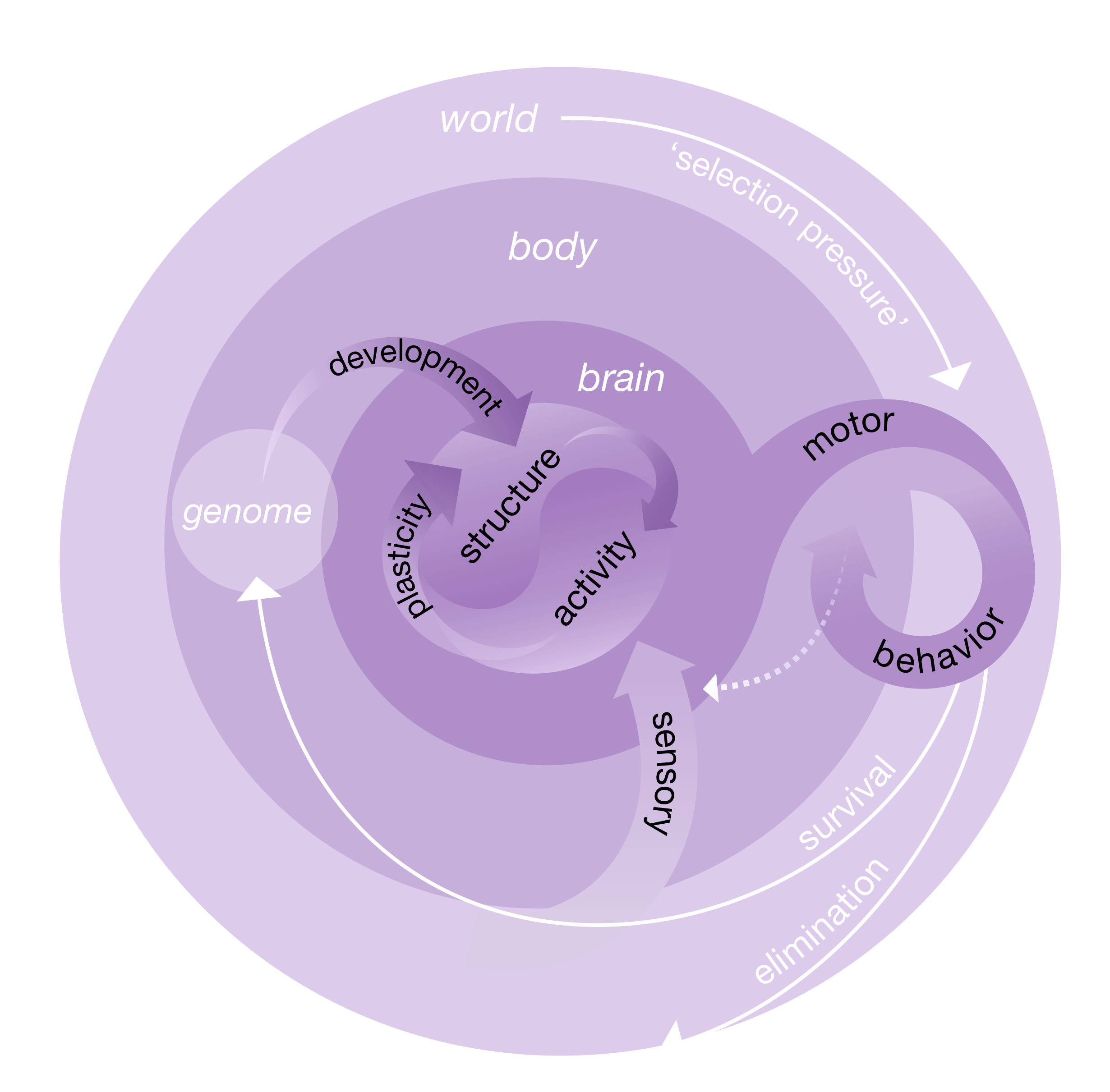
Figure 1: Scientific explanations, causal models, and dynamic systems all share a kind of structure. There are (1) parts, those parts have (2) properties and (3) activities which are (4) organized. In the above conceptual model, the parts are the brain, body, and world. The brain properties of interest is its structure (including its connectivity), and its activities include spiking and gene expression. Body properties include limbs, and its activities include both voluntary (such as movements) and involuntary (such as hearbeats and sensations). World properties include the environment in which the body interacts, its activities include other bodies, the rotation of the earth, etc. Brain activity causal impacts bodies, and bodies causally impact brains and world. For each individual, the initial condition is her genome. Image Credits: Julia Kuhl and Brett Mensh
The Connectome as a Model of Brain Structure
Brain structure is a complex multiscale abstraction characterizing many aspects of the brain. The connectome, as elaborated upon below, is our model of brain structure. The word “connectome” was independently coined in 2005 by both Professor Olaf Sporns and Dr. Patric Hagmann. Sporns defined the connectome as “a comprehensive structural description of the network elements and connections forming the human brain” (emphasis added).
The above definition leverages the concept from graph theory of a network, or graph. Any network is defined by two sets: a set of nodes (or vertices, or actors), and a set of edges (or arcs, or connections) between those nodes. Some networks are directed, meaning that edges communicate from one node to another, but not necessarily vice versa. Other networks are undirected, such that communication flows freely in both directions. Also, some networks are weighted, meaning that associated with each edge is a “strength”; otherwise, the network is binary, so edges are only “on” or “off”. Loops are allowed in some networks, meaning nodes can have edges with themselves. Finally, the graph, individual nodes, and edges may all have attributes. For examples, nodes may have labels, corresponding to which of several groups they participate in.
The connectome, according to this definition, can incorporate the entirety of brain structure, and it crucially includes connections between the elements. This is in stark contrast to typical discussions of anatomy, in which various morphological and functional properties of individual brain elements may be studied, but rarely connections between those elements. Since the original definitions, over 3000 publications have used the word “connectome”, and its meaning has expanded. Below, we provide our definition, which is an attempt to be as clear and concise as possible, while incorporating a wide net of its current usage.
- Definition A connectome is a network of a brain, at a particular spatiotemporal precision and extent. The nodes are biophysical (structrual) entities such as neurons, Brodmann areas, or voxels. The edges are either (1) structural, meaning they are physical objects, or (2) functional, meaning they characterize the statistical and/or causal relationship between the activity of a pair of nodes. The connectome as a whole, as well as each node and edge can have a rich set of attributes comprising its state space. For example, the connectome can have an overall volume, nodes can have complex morphological shapes, and edges can have many different proteins.
This definition implies that a given brain could have many different connectomes at different times, or at different resolutions, or of different types, etc. Given these choices, one can measure the parts of the brain to estimate their properties and activities. Linking back to the above approach to scientific explanation, we can therefore think of a connectome as a kind of explanation of the brain: the parts are the nodes, the activities characterize the kinds of edges, and the organization specifies which edges are present.
Example Connectomes
Figure 2 shows several different connectomes, to illustrate the flexibility of the connectome concept. Each is estimated from a different species spanning from the simplest to most complex animals, with widely disparate definitions of what consistutes nodes and edges.
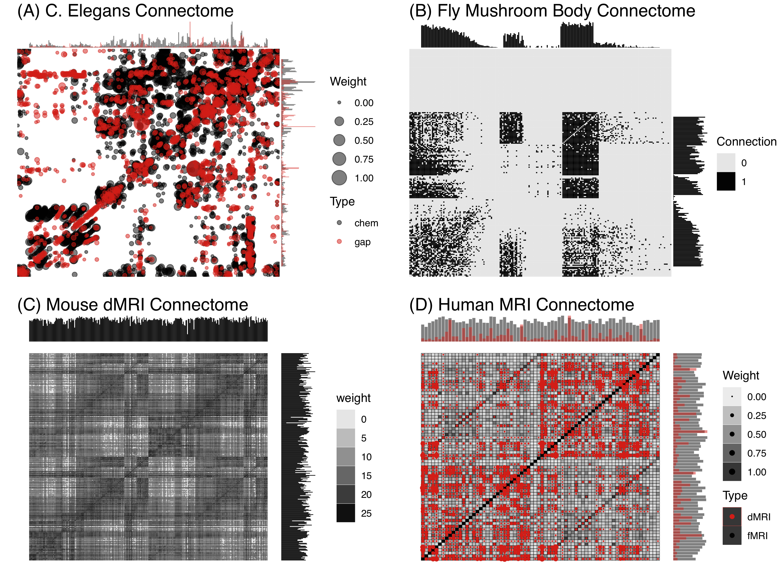
Figure 2 Connectomes spanning four levels of the phylogenetic tree, each acquired using different experimental modalities and spatial resolutions, ranging from nanoscale (electron microscopy) to macroscale (MRI regions). An adjacency matrix of a network shows the strength of connection between any pair of nodes. The connectomes are depicted as weighted adjacency matrices; for the worm and human, the connectomes are multi-connectomes, with two different edge types, denoted by two different colors. In each case, the nodes are sorted by region. Moreover, along each connectome we provide the degree sequence, that is, the sum of edge weights for each node.
-
(A) Caenorhabditis elegans The Caenorhabditis elegans (C. elegans) is the only animal that we have a complete connectome where the nodes represent neurons. It is complete in the sense that every neuron in the animal is a node, and every edge has been estimated. In this connectome, there are two types of edges corresponding to two types of neural activities: (1) chemical synapses, which correspond neurochemical release, and (2) gap junctions, which correspond to electrical activity. Each edge’s strength (or weight) corresponds to the number of synapses between its parent neurons. There are two sexes of C. elegans, the male and hermaphrodite, with different numbers of neurons (the male has more, most of the neurons are shared between the two sexes, but not all). These connectome estimates are derived by cumbersome manual tracing of axons and dendrites, and identification of synapses, in nanoscale electron micrographs, and were updated by Varshney et al. (2011) and Bentley (2016). The neurons have multiple kinds of labels, including names, side (left vs. right vs. neither) and class (sensory, internal, and motor). Figure 2(B) shows the hermaphrodite weighted multi-connectome, including both chemical (gray) and electrical (red) synapses. Note that chemical synapses are unidirectional, whereas electrical synapses are bidirectional.
-
(B) Drosophila melanogaster Eichler et al. (2017) published a complete larval Drosophila connectome of both the left and right mushroom body, also derived from serial electron microscopy, using only chemical synapses. These edges are weighted (based on counting the number of synapses between a pair of neurons), and directed. Neurons are categorized into kenyon cells (K), input neurons (I), output neurons (O), and projection neurons (P). Figure 2(B) shows both the left and right mushroom bodies. Edges are both weighted and directed.
-
(C) Mus musculus Calabrese et al. (2015) generated a high-resolution connectivity estimate using ex vivo diffusion magnetic resonance imaging (dMRI). This network is undirected, as dMRI lacks directional information, and weights correspond to the number of tracts estimated to go from one region to another. Because we do not know the mapping between the absolute magnitude of connection weights to any physical connection, we rescale these weights to be between zero and one, and depict them in Figure 2(C) on a log scale. Regions in the mouse connectome can be partitioned into “superstructures”, including frontal (F), hindbrain (H), midbrain (M), and white matter (W).
-
(D) Homo sapiens The Consortium for Reliability and Reproducibility collects multiple measurements of functional resting-state (F), anatomical (A), and/or diffusion (D) magnetic resonance imaging per individual. The functional connectomes are Pearson correlation matrices, which have been converted to ranks, and then normalized between zero and one, because such a representation has been shown to be more reliable than raw or thresholded correlations. The diffussion connectomes are normalized as described above for the mouse. The above multi-connectome estimate is derived from averaging the entire dataset consisting of 3,067 dMRI and 1,760 fMRI connectomes. Of the many possible brain parcellations, each defining nodes differently, we elected to use the Desikan parellation, assigning each cortical region into lobes including frontal (F), occiptal (O), parietal (P), and temporal (T), as well as sub-cortical structures (S).
What is and what is not, Connectomics?
In classical graph theory, nodes have no labels or other attributes, and neither do edges (including weights). Thus, commonly in connectomics the node labels, edge weights, and other properties are discarded during the analysis. Note, however, that there is no way to estimate a connectome without making decisions about which properties to incorporate, even if one can ignore them in the downstream analysis. However, the existing set of tools commonly used in connectomics does not incorporate these properties, thereby motivating extending the standard network analysis toolbox.
Note that we have not limited the definition of a connectome to be comprehensive set of all nodes and edges, because the concept of being comprehesive is not philosophically tenable. Even given the constraints of a particular spatial resolution and extent, the connectome varies over time, and various attributes could or could not be incorporated into the definition. In this case, referring to it as comprehensive is a bit vacuous, as it is only comprehensive relative to the imposed constraints, and everything is comprehensive with respect to some constraints. Thus, there does not exist a comprehensive connectome, even for an individual at a particular time. This is in stark contrast to an individual’s somatic genome, which is the genetic sequence of the mother cell of the individual. In genomics, each person really does have a single genome, and one can, in theory, estimate it with high accuracy. For this reason, calls to measure the “complete connectome” demand further elaboration and justification.
Connectomics differs from both classical anatomical studies and studies of neural circuitry. Typically, anatomical studies do not include studying connections between nodes, rather, they focus on the properties of each individual node. That said, connectomics, as mentioned above, requires some aspect of anatomy to define its nodes. Therefore, while all anatomical studies are not connectomics, all connectomics studies include anatomy. Similarly, it is not the case that all studies of neural circuitry are connectomics. In typical neural circuit investigations, the nodes are not distinct morphological objects, rather, they are abstractions, such as “all pyramidal cells in layer 4”. In this sense, not all studies of neural circuitry are connectomics, however, any study of connectomes may hope to reveal statistical principles that govern neural circuits. For example, studies on the somatic ganglion circuit of a crab, or the sound localization circuit of a barn owl were not connectomics. However, one could imagine a connectomics study of the same circuitry would reveal the same underlying principles.
Connectome Coding as an Approach to Learn About Connectomes
Connectome coding, as introduced here, is an approach to studying the brain that leverages connectomic data. To understand what connectome coding is requires understanding what a code is.
- Definition A code is a system of (potentially stochastic) rules that translate from one representation of information into another.
An example is the morse code, which is a system of rules that translate tones, lights, or clicks to alphanumeric characters. The morse code happens to be deterministic and “one-to-one” meaning that each sequence of beeps tranlate into a single character, and vice versa. The genetic code translates nucleotide triplets into amino acids. The genetic code is also deterministic, but it is not one-to-one, because multiple triplets encode the same nucleotide. The neural code translates between neural activity (typically spiking activity) and sensory input or motor output. This code is probabilistic, meaning that many different patterns of activity can encode the same stimulus or behavior, and a stimulus or behavior can elicit many different neural activity patterns. We are interested here in a different kind of code, which probabilistic governs connectomes.
-
Definition A connectome code is system of (potentially stochastic) rules that translate to and from connectomes.
In this sense, a genome encodes a connectome (and its dynamics via the rules of plasticity), and a connectome at any given time encodes the probability of various self-driven or responsive behaviors. There are therefore two kinds of connectome coding rules:
- connectome encoding rules translate from genomes to probabilities of (potentially dynamic) connectomes, and
- connectome decoding rules translate from connectomes to probabilities of (potentially dynamic) behaviors.
A Statistical Formalization of Connectome Coding
In the language of statistics, a code is a conditional distribution which characterizes the probability of an event conditioned on some other event. Statistical models consist of collections of random variables, each of which has parameters that govern its samples. Linking back to our approach to modeling, we say that each random variable is a “part”, its properties are the parameters of its distribution, and its activities are its potential realizations. The organization indicates which random variables are dependent on one another. Let , , and be random variables, their marginal distributions , , and characterize the probability of any particular , , or ; and their joint distribution characterizes the probability of observing and and . The conditional distribution characterizes the probability that takes a particular value given that is some value, and we can define other conditional distributions similarly. Our model will be dynamic, such that each random variable’s samples can change over time. Let therefore be the random variable for at time , and then (without a subscript) denotes the set of all ’s, . Finally, completely specifying any dynamical system requires also specifying initial conditions, in the form of a distribution characterizing .
In connectome coding, based on the above model, we have the following three random variables:
- brains, denoted by ,
- bodies, denoted by , and
- world, denoted by .
Thus, indicates the activity of the brain at time . Note that is a high dimensional object, because it corresponds to the entire brain at time . Each dimension of therefore represents the activity of a node in the brain network. In this sense, the parameters of the brain corresponds to brain structure, in other words, the connectome. Similarly, the parameters of the body correspond to body structure: bounds on strength, joint directions, etc., and parameters of the world correspond to world structure. The initial conditions for a given brain and body are specified by the somatic genome.
The art and practice of connectome coding therefore concerns estimating the statistical relationships between connectomes and genomes or behaviors. More specifically, connectome encoding is about learning the probability of given the genome. And connectome decoding is about learning the probability of behaviors given brain structure .
The above probabilistic description does not incorporate the concept of causality. However, our conceptual model does assert a causal structure. Specifically, the brain state at any time can impact future brain states, as well as future body states. The body state at any time can impact future brain, body, and world states. And the world state can impact future body states. Note that the world cannot directly impact the brain, without going through the body, and nothing can go backwards in time. The world state also determines, in collaboration with the body state of two individuals, the initial conditions for subsequent generation brain and body states. One of the implications of this causal dependence structure is that for the genome to encode the probabilistic rules of behavior to facilitate the organism winning the evolutionary game, it must go “through” the connectome. In other words, formalizing our conceptual model provides another perspective on the role of connectome codes: the causal mechanism connecting genes to brain activity and behavior requires going through a connectome. Since behavior is ongoing, dynamic, and responsive to the environment, and the somatic genome is static, the genome must essentially encode a blueprint that guides the construction of a vessel whose physical properties are such that they encourage “high value” behaviors. That vessel is the connectome. In other words, to get a desired phenotype, the genotype must specify the development of particular “connectotypes”. Note that the parameters of this model can also be time-varying, although that adds a level of complexity beyond the scope of this perspective.
This view of connectomes, connectome coding, and connectotyping, is, to our knowledge, essentially novel. That said, it is a conceptual and formal model that one can use to interpret any previous study of connectomics. Perhaps more important, we hope it will help guide the development and ideation of new connectomic studies, by providing a paradigm within which to ask, formalize, and eventually questions about neural circuit mechanisms, how they work, how they fail, and how they can be improved.
The above notes are based on an invited talk I gave at Baylor, and then a tutorial I gave at the Society for Neuroscience in 2017. More recently, I was asked to write an article for Current Opinion in Neurobology, which will be based largely on this blog post. This content flowed most recently from conversations with Brett Mensh, Carey E. Priebe, and Eric Bridgeford, who will be co-authors on the resulting manuscript. I presented a slide version of these contents at the Functional, Structural, and Molecular Imaging, and Big Data Analysis Short Course at SfN in 2018.